竟然画出椭圆了

import numpy as np
import matplotlib.pyplot as plt

if __name__ == "__main__":
    n = 1
    t = np.arange(0, 2 * np.pi * n, 0.01)
    r = 5

    x = r * np.cos(t) * 1.2
    y = r * np.sin(t)
    plt.plot(x, y)

    # 设置x,y坐标轴的刻度显示范围
    plt.xlim(-8, 8)
    plt.ylim(-8, 8)

    # 手动调整label顺序
    # handles, labels = plt.gca().get_legend_handles_labels()
    # order = [1, 0]
    # plt.legend([handles[idx] for idx in order], [labels[idx] for idx in order])
    # # 显示图例说明
    # plt.legend()

    # 获取当前坐标轴gca即get current axis
    ax = plt.gca()
    # 去掉上、右二侧的边框线
    ax.spines['top'].set_color('none')
    ax.spines['right'].set_color('none')
    # 将左侧的y轴，移到x=0的位置
    ax.spines['left'].set_position(('data', 0))
    # 将下面的x轴，移到y=0的位置
    ax.spines['bottom'].set_position(('data', 0))
    # 调整x轴刻度（从-5到+5，正好9个点）
    plt.xticks(np.linspace(-7, 7, 15))
    # 调整y轴刻度
    plt.yticks(np.linspace(-7, 7, 15))
    # 给纵坐标轴加箭头
    plt.arrow(0, 8, 0, 0, width=0.2, color="k", clip_on=False, head_width=0.2, head_length=0.2)
    # 给横坐标轴加箭头
    plt.arrow(8, 0, 0.01, 0, width=0.2, color="k", clip_on=False, head_width=0.2, head_length=0.2)

    plt.show()

椭圆2

import numpy as np
import matplotlib.pyplot as plt

if __name__ == "__main__":
    n = 1
    t = np.arange(0, 2 * np.pi * n, 0.01)
    r = 5

    x = r * np.cos(t + 1.2)
    y = r * np.sin(t)
    plt.plot(x, y)

    # 设置x,y坐标轴的刻度显示范围
    plt.xlim(-8, 8)
    plt.ylim(-8, 8)

    # 手动调整label顺序
    # handles, labels = plt.gca().get_legend_handles_labels()
    # order = [1, 0]
    # plt.legend([handles[idx] for idx in order], [labels[idx] for idx in order])
    # # 显示图例说明
    # plt.legend()

    # 获取当前坐标轴gca即get current axis
    ax = plt.gca()
    # 去掉上、右二侧的边框线
    ax.spines['top'].set_color('none')
    ax.spines['right'].set_color('none')
    # 将左侧的y轴，移到x=0的位置
    ax.spines['left'].set_position(('data', 0))
    # 将下面的x轴，移到y=0的位置
    ax.spines['bottom'].set_position(('data', 0))
    # 调整x轴刻度（从-5到+5，正好9个点）
    plt.xticks(np.linspace(-7, 7, 15))
    # 调整y轴刻度
    plt.yticks(np.linspace(-7, 7, 15))
    # 给纵坐标轴加箭头
    plt.arrow(0, 8, 0, 0, width=0.2, color="k", clip_on=False, head_width=0.2, head_length=0.2)
    # 给横坐标轴加箭头
    plt.arrow(8, 0, 0.01, 0, width=0.2, color="k", clip_on=False, head_width=0.2, head_length=0.2)

    plt.show()

竟然画出阿基米德螺旋线

import numpy as np
import matplotlib.pyplot as plt

if __name__ == "__main__":
    n = 4/5
    theta = np.arange(0, 2 * np.pi * n, 0.01)
    alpha = 3
    beta = 4
    r = alpha + beta * theta

    x = r * np.cos(theta)
    y = r * np.sin(theta)
    plt.plot(x, y)

    # 设置x,y坐标轴的刻度显示范围
    plt.xlim(-31, 31)
    plt.ylim(-31, 31)

    # 手动调整label顺序
    # handles, labels = plt.gca().get_legend_handles_labels()
    # order = [1, 0]
    # plt.legend([handles[idx] for idx in order], [labels[idx] for idx in order])
    # 显示图例说明
    # plt.legend()

    # 获取当前坐标轴gca即get current axis
    ax = plt.gca()
    # 去掉上、右二侧的边框线
    ax.spines['top'].set_color('none')
    ax.spines['right'].set_color('none')
    # 将左侧的y轴，移到x=0的位置
    ax.spines['left'].set_position(('data', 0))
    # 将下面的x轴，移到y=0的位置
    ax.spines['bottom'].set_position(('data', 0))
    # 调整x轴刻度（从-5到+5，正好9个点）
    plt.xticks(np.linspace(-30, 30, 11))
    # 调整y轴刻度
    plt.yticks(np.linspace(-30, 30, 11))
    # 给纵坐标轴加箭头
    plt.arrow(0, 31, 0, 0, width=0.2, color="k", clip_on=False, head_width=0.2, head_length=0.2)
    # 给横坐标轴加箭头
    plt.arrow(31, 0, 0.01, 0, width=0.2, color="k", clip_on=False, head_width=0.2, head_length=0.2)

    plt.show()

等高线画椭圆

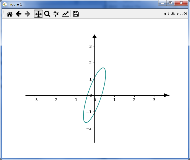
import matplotlib.pyplot as plt
import numpy as np

a, b = 7.79, 0.50
c, d = -4.50, 0.87


# 构造等高线函数
def f(x, y):
    return a * x ** 2 + b * x * y + c * y * x + d * y ** 2 - 1


# 定义点的数量
n = 500

# 作点
x = np.linspace(-3.5, 3.5, n)
y = np.linspace(-3.5, 3.5, n)

# 构造网格
X, Y = np.meshgrid(x, y)

# text方式的文本
# plt.text(-2, 1, r'$2x^2+(-1)xy+(-1)xy+2y^2=1$', fontdict={'size': 16, 'color': 'g'})

# 获取当前坐标轴gca即get current axis
ax = plt.gca()

# 去掉上、右二侧的边框线
ax.spines['top'].set_color('none')
ax.spines['right'].set_color('none')

# 将左侧的y轴，移到x=0的位置
ax.spines['left'].set_position(('data', 0))
ax.spines['bottom'].set_position(('data', 0))

# 调整x轴刻度（从-5到+5，正好11个点）
plt.xticks(np.linspace(-3, 3, 7))
# 调整y轴刻度
plt.yticks(np.linspace(-3, 3, 7))

# 给坐标轴加箭头
plt.arrow(0, 3.5, 0, 0, width=0.2, color="k", clip_on=False, head_width=0.2, head_length=0.2)
plt.arrow(3.5, 0, 0.01, 0, width=0.2, color="k", clip_on=False, head_width=0.2, head_length=0.2)


# 绘制等高线,8表示等高线数量加1
plt.contour(X, Y, f(X, Y), 0)
# plt.plot(x, y)
plt.show()

旋转矩阵的计算：

二阶矩阵相乘-20220621-手动横向输入-pre3

# 普通矩阵相乘
m, p, n = map(int, "2, 2, 2".split(","))  # 获得两个矩阵的行列数
A = []
B = []  # 创建A,B两个空列表，用以存放相乘的两个矩阵
C = [[0 for i in range(n)] for j in range(m)]  # 创建一个m行n列的初始化矩阵
print("请输入第1个矩阵：")
for i in range(1):
    A = list(map(float, (input().strip().split(" "))))  # 获得A矩阵

A1 = [A[0], A[1]]
A2 = [A[2], A[3]]
A = [A1, A2]

print("请输入第2个矩阵：")
for i in range(1):
    B = list(map(float, input().strip().split(" ")))  # 获得B矩阵

B1 = [B[0], B[1]]
B2 = [B[2], B[3]]
B = [B1, B2]

for i in range(m):
    for j in range(n):
        for k in range(p):
            C[i][j] += A[i][k] * B[k][j]  # 根据矩阵相乘的运算规则进行运算
for s in C:
    print()  # 保证输出为矩阵形式
    for r in s:
        print(r, end=" ")  # 输出结果矩阵

求一个二阶矩阵的逆矩阵-20220622-手动横向输入版-pre3

m, n = map(int, "2, 2".split(","))  # 获得两个矩阵的行列数
A = []
print("请输入一个矩阵：")
for i in range(1):
    A = list(map(float, (input().strip().split(" "))))  # 获得A矩阵

A1 = [A[0], A[1]]
A2 = [A[2], A[3]]
A = [A1, A2]

a = A[0][0]
b = A[0][1]
c = A[1][0]
d = A[1][1]

T1 = [a, b]
T2 = [c, d]

T = [T1, T2]

# print("初始矩阵是：")
# for s in T:
#     print()  # 保证输出为矩阵形式
#     for r in s:
#         print(r, end=" ")  # 输出结果矩阵
# print()

fenmu = a * d - b * c
# print("分母是：", fenmu)
T[0][0] = round(d / fenmu, 3)
T[0][1] = round(-b / fenmu, 3)
T[1][0] = round(-c / fenmu, 3)
T[1][1] = round(a / fenmu, 3)

print("\r\n\r\n其逆矩阵是：")
for s in T:
    print()  # 保证输出为矩阵形式
    for r in s:
        print(r, end=" ")  # 输出结果矩阵